Loading data
The load_data function takes in raw data and creates a
data object that can be accepted by the plot_design and
analyze functions. We use the made-up dataframe
sw_data_example to demonstrate the workflow.
data(sw_data_example)
head(sw_data_example)
#>   cluster period trt outcome_bin outcome_cont
#> 1       1      1   0           0  -3.02179837
#> 2       1      1   0           0  -0.07145287
#> 3       1      1   0           1   0.96807617
#> 4       1      1   0           0   0.29456948
#> 5       1      1   0           1  -0.83921584
#> 6       1      1   0           1  -0.42335941

dat <- load_data(
  time = "period",
  cluster_id = "cluster",
  individual_id = NULL,
  treatment = "trt",
  outcome = "outcome_bin",
  data = sw_data_example
)
#> Stepped wedge dataset loaded. Discrete time design with 15 clusters, 5 sequences, and 6 time points.
Plotting the design
The plot_design function produces a diagram of the
stepped wedge design and a summary of the variables.
plot_dat <- plot_design(dat)

print(plot_dat)
#> $design_plot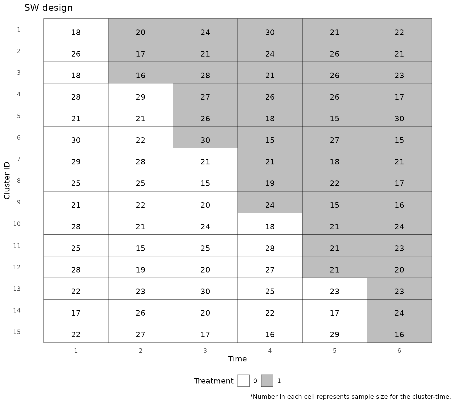
Analyzing the data
The analyze function analyzes the stepped wedge data.
First, we analyze the data using a mixed effects model, with the Time
Average Treament Effect (TATE) as the estimand, assuming an Immediate
Treatment (IT) effect, passing the family = "binomial" and
link = "logit" arguments to glmer. ## Binary
outcome
analysis_1 <- analyze(
  dat = dat,
  method = "mixed",
  estimand_type = "TATE",
  exp_time = "IT",
  family = binomial,
  re = c("clust", "time")
)

print(analysis_1)
#> Mixed model with random effects for cluster and time
#> Exp time: "IT", cal time: "categorical"
#> TATE (IT) estimate: 0.39
#> TATE (IT) 95% confidence interval: 0.123, 0.656
#> TATE (IT) p-value: 0.0041307
#> Converged: TRUE
Repeat the analysis, but including a random effect for cluster only, not for cluster-time interaction.
analysis_1b <- analyze(
  dat = dat,
  method = "mixed",
  estimand_type = "TATE",
  exp_time = "IT",
  family = binomial,
  re = "clust"
)

print(analysis_1b)
#> Mixed model with random effects for cluster
#> Exp time: "IT", cal time: "categorical"
#> TATE (IT) estimate: 0.391
#> TATE (IT) 95% confidence interval: 0.128, 0.653
#> TATE (IT) p-value: 0.0035093
#> Converged: TRUE
Repeat the analysis, but using GEE rather than a mixed model.
analysis_2 <- analyze(
  dat = dat,
  method = "GEE",
  estimand_type = "TATE",
  exp_time = "IT",
  family = binomial,
  corstr = "exchangeable"
)

print(analysis_2)
#> GEE model with working exchangeable correlation structure
#> Exp time: "IT", cal time: "categorical"
#> TATE (IT) estimate: 0.389
#> TATE (IT) 95% confidence interval: 0.138, 0.64
#> TATE (IT) p-value: 0.0024142
#> Converged: NA
Mixed model, with Time Average Treament Effect (TATE) as the estimand, using an Exposure Time Indicator (ETI) model.
analysis_3 <- analyze(
  dat = dat,
  method = "mixed",
  estimand_type = "TATE",
  exp_time = "ETI",
  family = binomial
)

print(analysis_3)
#> Mixed model with random effects for cluster and time
#> Exp time: "ETI", cal time: "categorical"
#> TATE estimate: 0.418
#> TATE 95% confidence interval: 0.102, 0.733
#> TATE p-value: 0.0094832
#> Converged: TRUE
Mixed model, with Time Average Treatment Effect (TATE) as the estimand, using a Natural Cubic Splines (NCS) model.
analysis_4 <- analyze(
  dat = dat,
  method = "mixed",
  estimand_type = "TATE",
  exp_time = "NCS",
  family = binomial
)

print(analysis_4)
#> Mixed model with random effects for cluster and time
#> Exp time: "NCS", cal time: "categorical"
#> TATE estimate: 0.421
#> TATE 95% confidence interval: 0.104, 0.738
#> TATE p-value: 0.0092387
#> Converged: TRUE
Mixed model using a Delayed Constant Treatment (DCT) model. This
model assumes the treatment effect during the first w
exposure time periods is a nuisance “washout” effect, after which the
treatment stabilizes to a constant effect
.
Set w via params().
analysis_5 <- analyze(
  dat = dat,
  method = "mixed",
  estimand_type = "TATE",
  exp_time = "DCT",
  family = binomial,
  advanced = params(w = 2)
)

print(analysis_5)
#> Mixed model with random effects for cluster and time
#> Exp time: "DCT", cal time: "categorical"
#> TATE (DCT) estimate: 0.321
#> TATE (DCT) 95% confidence interval: -0.05, 0.692
#> TATE (DCT) p-value: 0.089915
#> Converged: TRUE
The returned te_est is the estimate of
— the constant treatment effect after the washout period. The
washout-period coefficients
()
are estimated internally but treated as nuisance parameters.
Continuous outcome
Mixed model, with Time Average Treament Effect (TATE) as the estimand, using a Natural Cubic Splines (NCS) model.
dat_cont <- load_data(
  time = "period",
  cluster_id = "cluster",
  individual_id = NULL,
  treatment = "trt",
  outcome = "outcome_cont",
  data = sw_data_example
)
#> Stepped wedge dataset loaded. Discrete time design with 15 clusters, 5 sequences, and 6 time points.

analysis_6 <- analyze(
  dat = dat_cont,
  method = "mixed",
  estimand_type = "TATE",
  exp_time = "NCS",
  family = gaussian
)

print(analysis_6)
#> Mixed model with random effects for cluster and time
#> Exp time: "NCS", cal time: "categorical"
#> TATE estimate: 0.526
#> TATE 95% confidence interval: 0.329, 0.723
#> TATE p-value: < 0.001
#> Converged: TRUE
Binomial outcome
When loading data where the outcome is binomial, specify the names of
the “# of successes” and “# of trials” variables as the
outcome argument.
dat_binom <- load_data(
  time ="period",
  cluster_id = "cluster",
  individual_id = NULL,
  treatment = "trt",
  outcome = c("numerator", "denominator"),
  data = sw_data_example_binom
)
#> Stepped wedge dataset loaded. Discrete time design with 15 clusters, 5 sequences, and 6 time points.
Mixed model, with Time Average Treament Effect (TATE) as the estimand, using an Exposure Time Indicator (ETI) model.
analysis_binom <- analyze(
  dat = dat_binom,
  method = "mixed",
  family = binomial,
  estimand_type = "TATE",
  exp_time = "ETI")
#> boundary (singular) fit: see help('isSingular')

print(analysis_binom)
#> Mixed model with random effects for cluster and time
#> Exp time: "ETI", cal time: "categorical"
#> TATE estimate: 0.696
#> TATE 95% confidence interval: 0.397, 0.996
#> TATE p-value: < 0.001
#> Converged: FALSE
Plotting effect curves
The plot_effect_curve function plots effect estimates by
exposure time for one or more analyze objects.
IT_model <- analyze(
  dat = dat_cont, method = "mixed", estimand_type = "TATE",
  estimand_time = c(1, 4), exp_time = "IT"
)
ETI_model <- analyze(
  dat = dat_cont, method = "mixed", estimand_type = "TATE",
  estimand_time = c(1, 4), exp_time = "ETI"
)
NCS_4_model <- analyze(
  dat = dat_cont, method = "mixed", estimand_type = "TATE",
  estimand_time = c(1, 4), exp_time = "NCS",
  advanced = params(n_knots_exp = 4)
)
DCT_model <- analyze(
  dat = dat_cont, method = "mixed", estimand_type = "TATE",
  estimand_time = c(1, 4), exp_time = "DCT",
  advanced = params(w = 2)
)

plot_effect_curves(IT_model, ETI_model, NCS_4_model, DCT_model, facet_nrow = 2)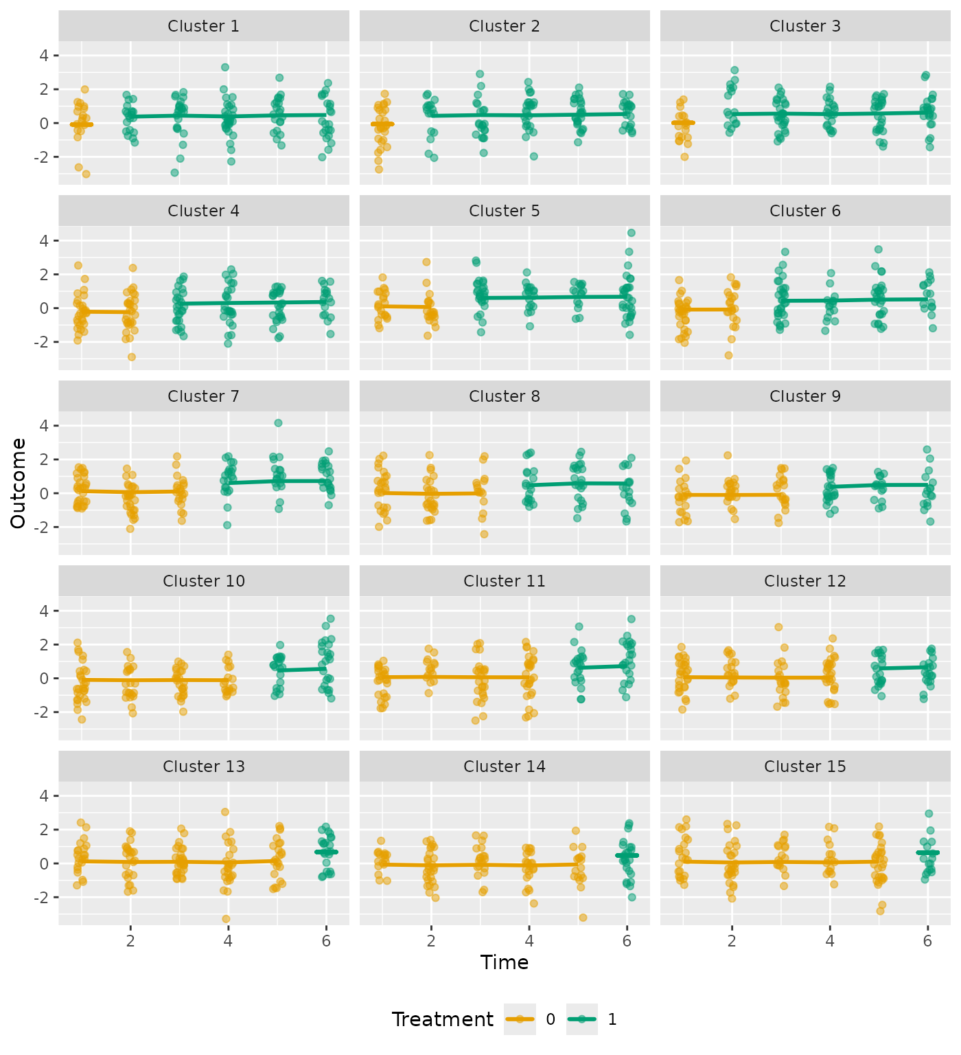
Plotting cluster charts
The plot_clusters function plots actual and predicted
outcomes for each cluster by calendar time for an analyze
object.
Continuous outcome
For continuous outcomes, the actual outcomes are jittered, with the predicted outcomes represented by the plotted line:
plot_clusters(analysis_6, ncol = 3)
#> $cluster_chart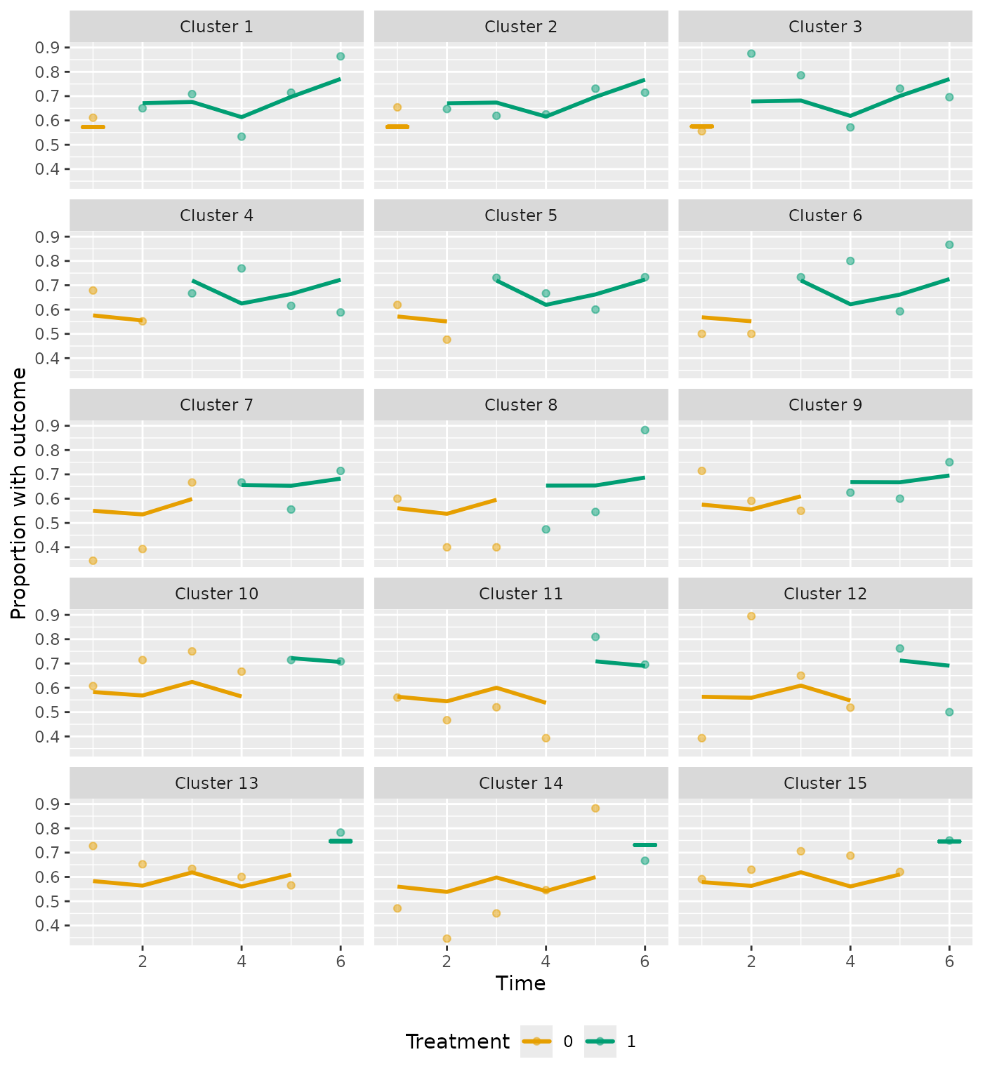
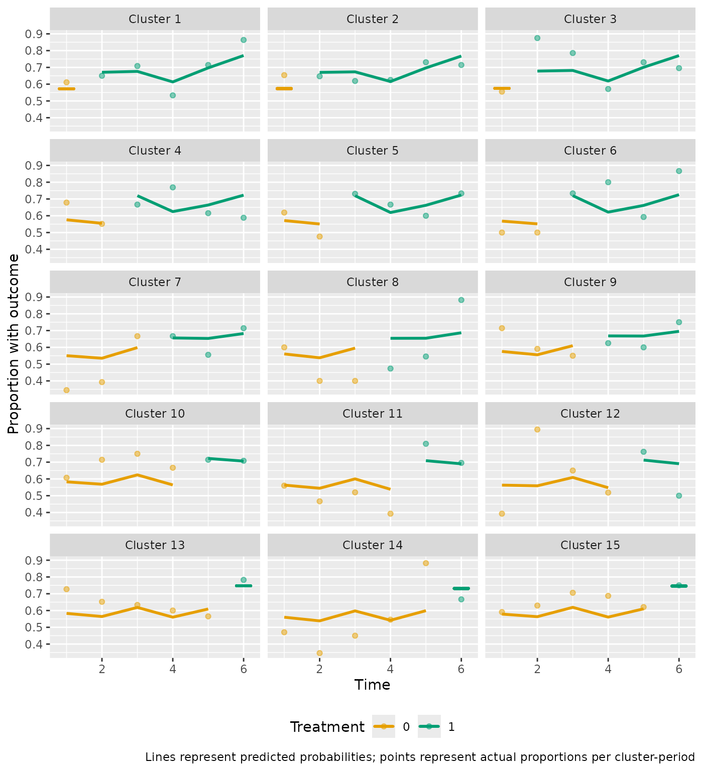
Binary outcome
For binary outcomes, the observed probability for each cluster period is plotted as a point, with the predicted probabilities represented by the plotted line:
plot_clusters(analysis_4, ncol = 3)
#> $cluster_chart