When developing a novel statistical method, we often wish to compare our proposed method with one or more existing methods. This serves to highlight the differences between our method and whatever is used in common practice. Generally, we wish to examine realistic settings, motivated by statistical theory, in which the novel method confers some advantage over the alternatives.
In this example, we will consider the problem of estimating the variance-covariance matrix of the least-squares estimator in linear regression. We assume the reader has some familiarity with linear regression.
Suppose our dataset consists of independent observations , where and are both scalar variables. A general linear regression model posits that
where is a mean-zero noise term with variance . We refer to this as a heteroskedastic model, since the variances need not be equal across all . This is the true data-generating model. (Note: A more restrictive (but misspecified) model assumes that there is a common variance such that for all . We refer to this incorrect model as the homoskedastic model.)
In linear regression, we use least-squares to estimate the
coefficient vector
.
For the purposes of building confidence intervals and performing
hypothesis tests, we need to also estimate the standard error of the
least squares estimator. There are two common ways to do this: (1) Use a
model-based standard error that assume homoskedasticity. This is the
estimator used by default in most statistical software (including the
lm function in R). (2) Use a so-called sandwich standard
error. Statistical theory tells us that estimator will be consistent
even under heteroskedasticity. See the Statistical Appendix for more
details.
We will carry out a small simulation study to compare these two estimators.
We start by declaring a new simulation object and writing a function that generates some data according to our model. For this simulation, we will make larger for larger values of .
sim <- new_sim()

create_regression_data <- function(n) {
  beta <- c(-1, 10)
  x <- rnorm(n)
  sigma2 <- exp(x)
  y <- rnorm(n=n, mean=(beta[1]+beta[2]*x), sd = sqrt(sigma2))
  return(data.frame(x=x, y=y))
}
To get a sense of what heteroskedasticity looks like in practice, we can generate a dataset, fit a linear regression model, and make a scatterplot of the residuals against .
dat <- create_regression_data(n=500)
linear_model <- lm(y~x, data=dat)
dat$residuals <- linear_model$residuals

library(ggplot2)
ggplot(dat, aes(x=x, y=residuals)) +
  geom_point() +
  theme_bw() +
  labs(x="x", y="residual")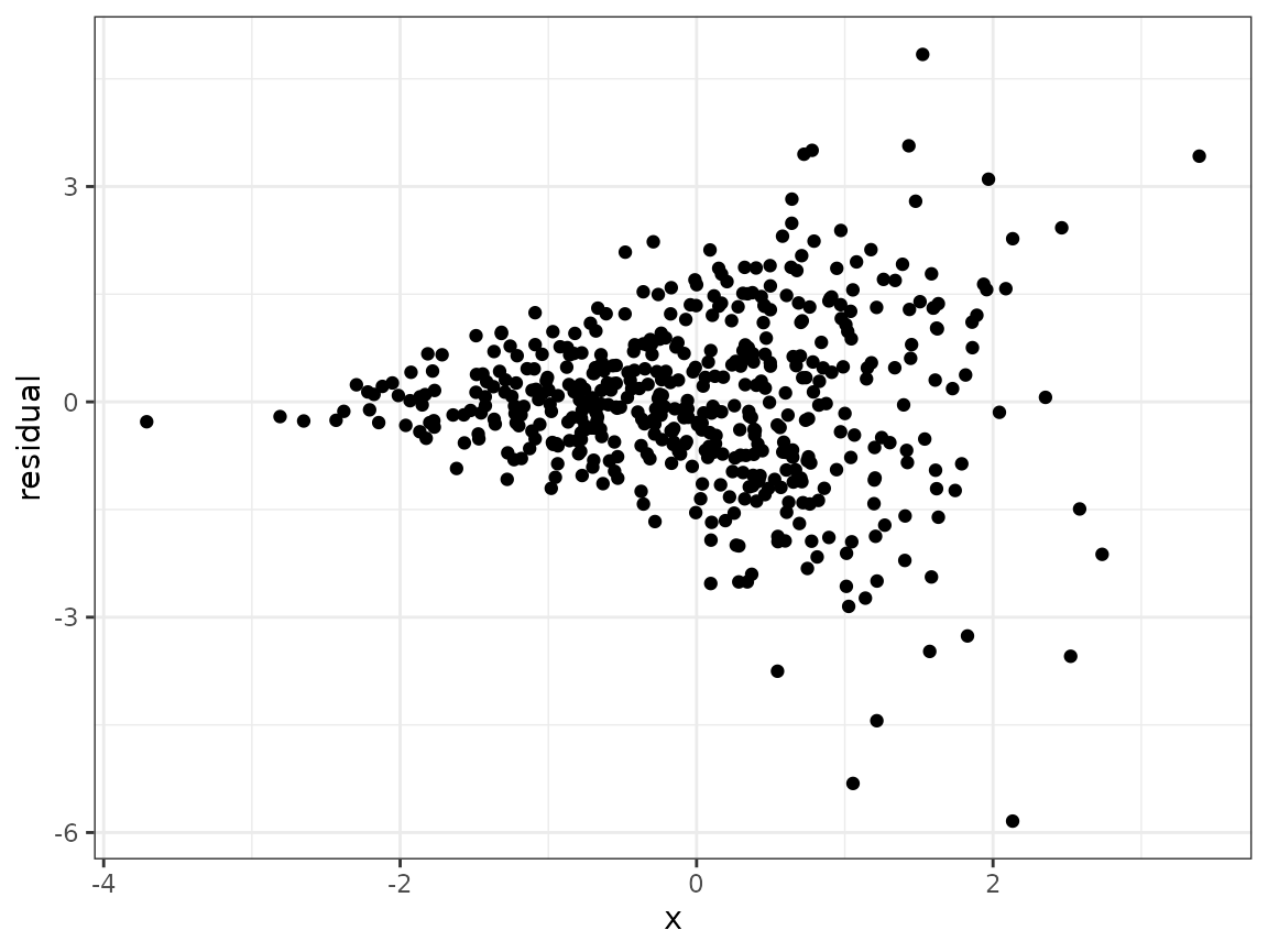
Now we declare two methods: one returns the least squares estimate and model-based estimator of the variance-covariance matrix of , and the other returns the least squares estimate and sandwich estimator (using the sandwich package).
model_vcov <- function(data) {
  mod <- lm(y~x, data=data)
  return(list("coef"=mod$coefficients, "vcov"=diag(vcov(mod))))
}

sandwich_vcov <- function(data) {
  mod <- lm(y~x, data=data)
  return(list("coef"=mod$coefficients, "vcov"=diag(vcovHC(mod))))
}
Next, we write the simulation script. This script returns a point
estimate and a standard error estimate for both the intercept parameter
and the slope parameter
.
We will tell SimEngine to run 500 simulation replicates for each of four
sample sizes. It is important to use the seed argument in
set_config so that our results will be reproducible. In
addition, we will use the packages option to load the
sandwich package. Loading packages via set_config (as
opposed to running library(sandwich)) is required if
running simulations in parallel. Finally, we run the simulation.
sim %<>% set_script(function() {
  data <- create_regression_data(n=L$n)
  estimates <- use_method(L$estimator, list(data))
  return(list(
    "beta0_est" = estimates$coef[1],
    "beta1_est" = estimates$coef[2],
    "beta0_se_est" = sqrt(estimates$vcov[1]),
    "beta1_se_est" = sqrt(estimates$vcov[2])
  ))
})

sim %<>% set_levels(
  estimator = c("model_vcov", "sandwich_vcov"),
  n = c(50, 100, 500, 1000)
)

sim %<>% set_config(
  num_sim = 500,
  seed = 24,
  packages = c("sandwich")
)

sim %<>% run()
#> Done. No errors or warnings detected.
Now we can summarize the results using summarize. There
are two main quantities of interest for us. The primary purpose of the
standard error estimate for
is to form confidence intervals, so we will look at (1) the average
width of the resulting interval (simply 1.96 times the average standard
error estimate across simulation replicates), and (2) the estimated
coverage of the interval, which is simply the proportion of simulation
replicates in which the interval contains the true value of
.
We will focus on 95% confidence intervals in this simulation.
summarized_results <- sim %>% summarize(
  list(stat="mean", name="mean_se_beta0", x="beta0_se_est"),
  list(stat="mean", name="mean_se_beta1", x="beta1_se_est"),
  list(stat="coverage", name="cov_beta0", estimate="beta0_est",
       se="beta0_se_est", truth=-1),
  list(stat="coverage", name="cov_beta1", estimate="beta1_est",
       se="beta1_se_est", truth=10)
)

print(summarized_results)
#>   level_id     estimator    n n_reps mean_se_beta0 mean_se_beta1 cov_beta0
#> 1        1    model_vcov   50    500    0.18100830    0.18233202     0.946
#> 2        2 sandwich_vcov   50    500    0.18235693    0.24320294     0.938
#> 3        3    model_vcov  100    500    0.12724902    0.12778192     0.946
#> 4        4 sandwich_vcov  100    500    0.12805679    0.17341936     0.942
#> 5        5    model_vcov  500    500    0.05704424    0.05697317     0.946
#> 6        6 sandwich_vcov  500    500    0.05748439    0.07960900     0.948
#> 7        7    model_vcov 1000    500    0.04055718    0.04059151     0.960
#> 8        8 sandwich_vcov 1000    500    0.04052126    0.05721446     0.958
#>   cov_beta1
#> 1     0.848
#> 2     0.922
#> 3     0.862
#> 4     0.946
#> 5     0.836
#> 6     0.940
#> 7     0.860
#> 8     0.958
To visualize our results, we set up a plotting function.
library(tidyr)
#>
#> Attaching package: 'tidyr'
#> The following object is masked from 'package:magrittr':
#>
#>     extract
plot_results <- function(which_graph, n_est) {
  if (n_est == 3) {
    values <- c("#999999", "#E69F00", "#56B4E9")
    breaks <- c("model_vcov", "sandwich_vcov", "bootstrap_vcov")
    labels <- c("Model-based", "Sandwich", "Bootstrap")
  } else {
    values <- c("#999999", "#E69F00")
    breaks <- c("model_vcov", "sandwich_vcov")
    labels <- c("Model-based", "Sandwich")
  }
  if (which_graph == "width") {
    summarized_results %>%
    pivot_longer(
      cols = c("mean_se_beta0", "mean_se_beta1"),
      names_to = "parameter",
      names_prefix = "mean_se_"
    ) %>%
    dplyr::mutate(value_j = jitter(value, amount = 0.01)) %>%
    ggplot(aes(x=n, y=1.96*value_j, color=estimator)) +
    geom_line(aes(linetype=parameter)) +
    geom_point() +
    theme_bw() +
    ylab("Average CI width") +
    scale_color_manual(
      values = values,
      breaks = breaks,
      name = "SE estimator",
      labels = labels
    ) +
    scale_linetype_discrete(
      breaks = c("beta0", "beta1"),
      name = "Parameter",
      labels = c(expression(beta[0]), expression(beta[1]))
    )
  } else {
    summarized_results %>%
    pivot_longer(
      cols = c("cov_beta0","cov_beta1"),
      names_to = "parameter",
      names_prefix = "cov_"
    ) %>%
    dplyr::mutate(value_j = jitter(value, amount = 0.01)) %>%
    ggplot(aes(x=n, y=value, color=estimator)) +
    geom_line(aes(linetype = parameter)) +
    geom_point() +
    theme_bw() +
    ylab("Coverage") +
    scale_color_manual(
      values = values,
      breaks = breaks,
      name = "SE estimator",
      labels = labels
    ) +
    scale_linetype_discrete(
      breaks = c("beta0", "beta1"),
      name = "Parameter",
      labels = c(expression(beta[0]), expression(beta[1]))
    ) +
    geom_hline(yintercept=0.95)
  }
}
We then use the plotting function to make our figures.
plot_results("width", 2)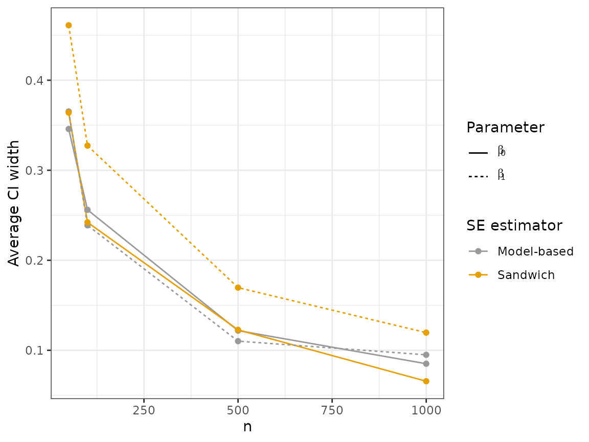
plot_results("coverage", 2)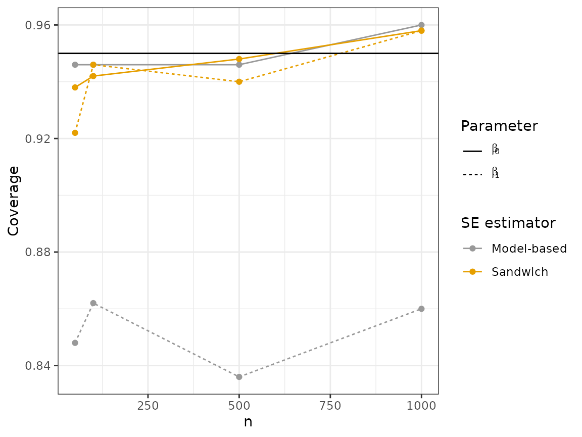
Looking at these plots, we can see that the sandwich method results in a wider interval, on average, for . In terms of coverage, the sandwich estimator achieves near nominal coverage for both parameters, while there is moderate undercoverage for using the model-based estimator.
The bootstrap is another popular approach to estimating standard
errors. We can add a bootstrap method and use update_sim to
run the new simulation replicates without re-running any of our previous
work. All we need to do is include the new estimator in our simulation
levels. Since the bootstrap can be computationally intensive, we will
use parallelization to speed things up. This requires us to specify the
option parallel = TRUE in set_config. (Even
with parallelization, update_sim will likely take a few
minutes to run.)
bootstrap_vcov <- function(data) {
  mod <- lm(y~x, data=data)
  boot_ests <- matrix(NA, nrow=100, ncol=2)
  for (j in 1:100) {
    indices <- sample(1:nrow(data), size=nrow(data), replace=TRUE)
    boot_dat <- data[indices,]
    boot_mod <- lm(y~x, data=boot_dat)
    boot_ests[j,] <- boot_mod$coefficients
  }
  boot_v1 <- var(boot_ests[,1])
  boot_v2 <- var(boot_ests[,2])
  return(list("coef"=mod$coefficients, "vcov"=c(boot_v1, boot_v2)))
}

sim %<>% set_levels(
  estimator = c("model_vcov", "sandwich_vcov", "bootstrap_vcov"),
  n = c(50, 100, 500, 1000)
)

sim %<>% set_config(
  num_sim = 500,
  seed = 24,
  parallel = TRUE,
  n_cores = 2,
  packages = c("sandwich")
)

sim %<>% update_sim()
#> Done. No errors or warnings detected.
Now that we have the bootstrap results included in our simulation object, we can look at the updated results.
summarized_results <- sim %>% summarize(
  list(stat="mean", name="mean_se_beta0", x="beta0_se_est"),
  list(stat="mean", name="mean_se_beta1", x="beta1_se_est"),
  list(stat="coverage", name="cov_beta0", estimate="beta0_est",
       se="beta0_se_est", truth=-1),
  list(stat="coverage", name="cov_beta1", estimate="beta1_est",
       se="beta1_se_est", truth=10)
)

plot_results("width", 3)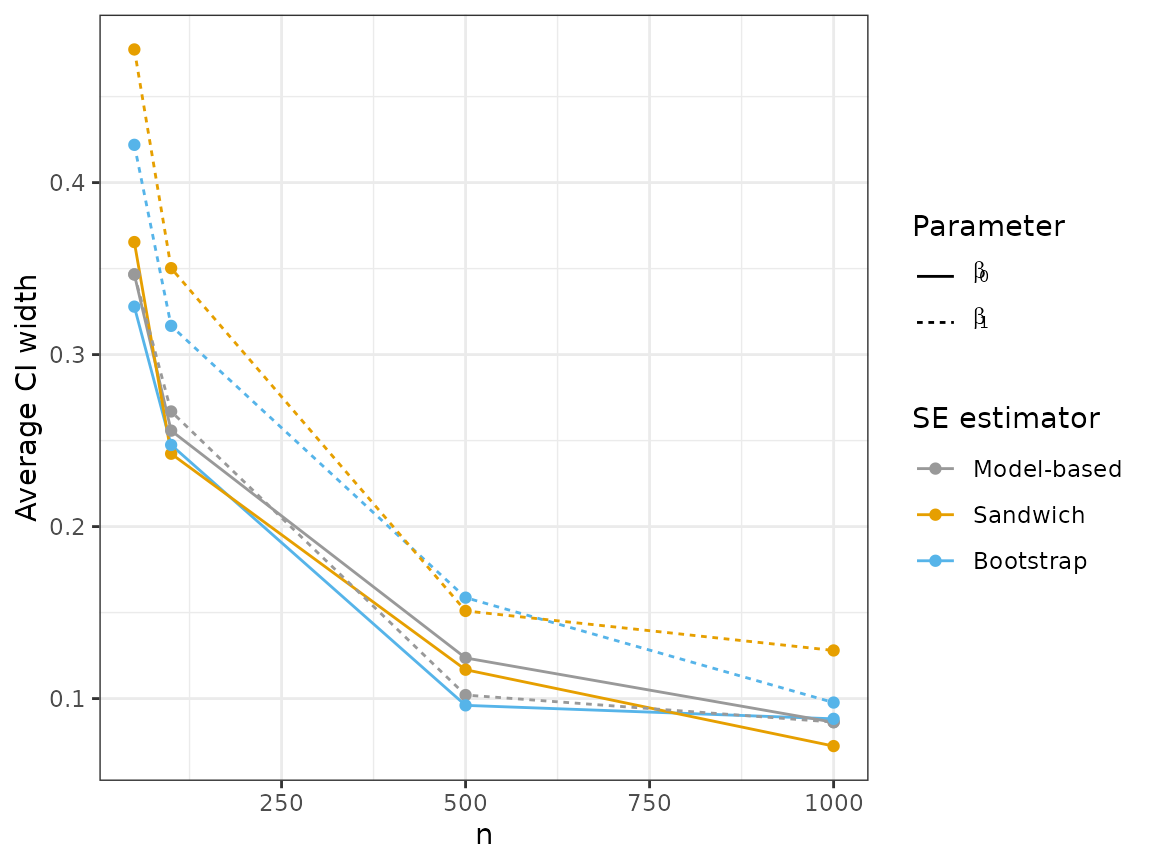
plot_results("coverage", 3)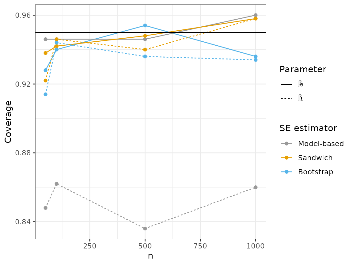
Like the sandwich estimator, the bootstrap results in wider intervals for , but is much closer to achieving 95% coverage compared to the model-based estimator.
Statistical appendix
For notational simplicity, we build a matrix , whose first column is all 1’s (the intercept column) and whose second column is . We also define a matrix
The ordinary least squares estimator of is . The variance of this estimator, which we call is
The usual estimator of is the model-based standard error , where . However, under our heteroskedastic model where the are not all equal, this is not a consistent estimator of ! That is to say, even in large samples, we cannot generally expect this estimator to be close to the truth.
A better estimator for our setting is the sandwich standard error, or Huber-White standard error, given by
where
